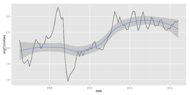
For each Augmented Dickey-Fuller (ADF) test looking for unit root, done using the ur.df() function within the urca package, I am including a graph of that variable as a visual reference:
1. The averaged price of U.S. Conventional Gasoline prices
> gasADFtest <- summary(ur.df(avgConvGas,
type = "drift",
selectlags = "BIC"))
> gasADFtest

###############################################
# Augmented Dickey-Fuller Test Unit Root Test #
###############################################

Test regression drift


Call:
lm(formula = z.diff ~ z.lag.1 + 1 + z.diff.lag)

Residuals:
     Min       1Q   Median       3Q      Max
-1.08395 -0.10528  0.01245  0.13314  0.31021

Coefficients:
            Estimate Std. Error t value Pr(>|t|)
(Intercept)  0.24809    0.08949   2.772  0.00675 **
z.lag.1     -0.10241    0.03706  -2.764  0.00692 **
z.diff.lag   0.39773    0.09582   4.151 7.45e-05 ***
---
Signif. codes:  0 ‘***’ 0.001 ‘**’ 0.01 ‘*’ 0.05 ‘.’ 0.1 ‘ ’ 1

Residual standard error: 0.1941 on 91 degrees of freedom
Multiple R-squared:  0.1881, Adjusted R-squared:  0.1703
F-statistic: 10.54 on 2 and 91 DF,  p-value: 7.616e-05


Value of test-statistic is: -2.7637 3.8806

Critical values for test thestatistics:
      1pct  5pct 10pct
tau2 -3.51 -2.89 -2.58
phi1  6.70  4.71  3.86
2. The West Texas Intermediate crude oil spot price
> wtiADFtest <- summary(ur.df(wti,
type = "drift",
selectlags = "BIC"))
> wtiADFtest

###############################################
# Augmented Dickey-Fuller Test Unit Root Test #
###############################################

Test regression drift


Call:
lm(formula = z.diff ~ z.lag.1 + 1 + z.diff.lag)

Residuals:
     Min       1Q   Median       3Q      Max
-0.47603 -0.08486  0.01266  0.10034  0.34917

Coefficients:
            Estimate Std. Error t value Pr(>|t|)
(Intercept)  0.19902    0.07044   2.825  0.00580 **
z.lag.1     -0.09557    0.03394  -2.816  0.00596 **
z.diff.lag   0.47096    0.09296   5.066 2.11e-06 ***
---
Signif. codes:  0 ‘***’ 0.001 ‘**’ 0.01 ‘*’ 0.05 ‘.’ 0.1 ‘ ’ 1

Residual standard error: 0.147 on 91 degrees of freedom
Multiple R-squared:  0.2432, Adjusted R-squared:  0.2265
F-statistic: 14.62 on 2 and 91 DF,  p-value: 3.123e-06


Value of test-statistic is: -2.8159 4.0264

Critical values for test statistics:
      1pct  5pct 10pct
tau2 -3.51 -2.89 -2.58
phi1  6.70  4.71  3.86
3. The Brent crude oil spot price
> brentADFtest <- summary(ur.df(brent,
type = "drift",
selectlags = "BIC"))
> brentADFtest

###############################################
# Augmented Dickey-Fuller Test Unit Root Test #
###############################################

Test regression drift


Call:
lm(formula = z.diff ~ z.lag.1 + 1 + z.diff.lag)

Residuals:
     Min       1Q   Median       3Q      Max
-0.42331 -0.07683  0.02460  0.10103  0.35226

Coefficients:
            Estimate Std. Error t value Pr(>|t|)
(Intercept)  0.14981    0.06196   2.418   0.0176 *
z.lag.1     -0.06661    0.02777  -2.399   0.0185 *
z.diff.lag   0.48010    0.09208   5.214 1.15e-06 ***
---
Signif. codes:  0 ‘***’ 0.001 ‘**’ 0.01 ‘*’ 0.05 ‘.’ 0.1 ‘ ’ 1

Residual standard error: 0.147 on 91 degrees of freedom
Multiple R-squared:  0.2468, Adjusted R-squared:  0.2302
F-statistic: 14.91 on 2 and 91 DF,  p-value: 2.509e-06


Value of test-statistic is: -2.399 2.9484

Critical values for test statistics:
      1pct  5pct 10pct
tau2 -3.51 -2.89 -2.58
phi1  6.70  4.71  3.86
Based on reviewing the visualized graphs, I chose to use the type = "drift" option in the ur.df() function. I do not believe that any strong signs of a trend exist in the data, but I do believe that it is appropriate to treat it for a drift term. I also used the Bayesian information criteria in order to select the lags used with the selectlags = "BIC" option -- which selected a lag of one (1) for the ADF test.
For each variable, the ADF test shows that we can not reject the null hypothesis that the variable has a unit root. At the bottom of each test is the ADF test statistic and the ADF test critical values. In all cases, we can not reject the null hypothesis at the 5-percent significance level, labeled 5pct, and only for the average gasoline price and the WTI crude price are they significant at the 10-percent (10pct) significance level. For the purposes of my research and this blog post, I am going to assume that each variable exhibits has a unit root. The regressions in each test shows the significance of the intercept, lagged term, and the drift component, all of which are statistically significant within the 5-percent significance level.
From here, I will continue my research using the first difference of each variable. The plots below are for each variable, now in a first-difference form.:
These first-differenced variables make the data stationary about a mean of zero (or near to it, which can be checked by summarizing the variables with summary()) and will aid in performing an accurate causal analysis, which I will perform in my next post. I plan to conclude this series with my next blog post and make a final update to my GitHub repository for this work as well as list the works I used in the course of my original research, when this was my thesis project.


