U.S. Presidential Election Participation

After a substantial pause in my blogging, I am back at it.

Another presidential election cycle is in full swing here in the United States.  In between all of the arguing of which candidate is the best choice -- or the lesser evil -- I have heard and read people talking about polling numbers and previous election results.

"Hillary has X% of Americans supporting her!"

"Trump should receive Y% of the votes!"

All of this got me thinking about a debate with some friends about voter turnout.  The point that I brought up then, and will be publishing here, is the stagnant participation rate for voting in the United States.

In this first graph, I have charted out the U.S. population estimates as calculated by the U.S. Census Bureau, making presidential election years my observation points:

The solid black line is the estimated total U.S. population.  The red dot-dash line beneath it is the estimated U.S. voting-aged population.  Finally, the blue dashed line at the bottom is the count of the U.S. population that actually voted.  What stands out is the difference between the rate of increase in the population and the rate of of increase in those that vote.

This next graph shows the percentage of voting-aged population to the total population (top, sold blank line) and the percentage of those who voted to the total population (bottom, red dot-dash line).

It appears that the proportion of the population that votes is stable (stagnant?) when compared to the increase in the proportion of the population estimated to be of voting-age in the United States.  Finally, to conclude this post on demographics, below is the percent of voting-aged population that actually votes.  There is some volatility but it appears to be declining over time.

I have no preference in this year's election.  I may actually join the ranks of those who fail to vote... who knows?  And, while I think we will see a slight increase in voter participation in this election cycle, I think that the disturbing trend of decreasing voter participation will continue over the long term.

As usual, I will make the data and the R script used in this post available in my GitHub repository.

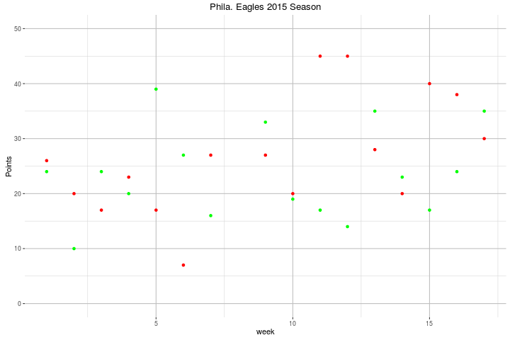
I will start working on my next post with the goal of returning my focus to economic topics, but you never know... the Philadelphia Eagles are looking pretty good this season.

A Brief Update

I mistakenly thought I would have time to blog, and I apologize to anyone who has been waiting for me to post something new to read.  Life, both personal and professional, has been going well but has also been extremely busy.

One thing that I would like to comment on before I go any further is the progress I have made through Coursera.  I have been taking courses in both the Data Science specialization track (here) and in the Python for Everybody track (here).

The Data Science track, offered by Johns Hopkins University, has been a great hands-on crash course for using R -- something I have been playing with for years, but never went much further than creating some basic visualizations.  Right now, I am finishing up the certificate program with the capstone project course which combines lessons from the previous courses and adds a twist: performing some Natural Language Processing (NLP).  For this project, JHU/Coursera has partnered with SwiftKey to make data available to the students and provide some background on how NLP works.

The Python for Everybody track has been a great experience with learning Python, especially since my programming skills were pretty minimal.  This is offered through University of Michigan and taught by Dr. Chuck Severance.  So far, I have completed the first three courses in the series.  I have gotten a decent grasp of the basics of using Python, and I am looking forward to using it more while performing data analysis.

Now for the future of this blog.  It shall continue.  I am currently working on two posts: one going back to my interest in oil prices and the other visualizing some macroeconomic variables (interest rates, stock market values, etc.) in the global market.  I plan on having at least one posted next month, as soon as I complete my capstone project.

Thank you for your patience and understanding.

A Quick Look At The Philadelphia Eagles 2015 Season

Now that I have some time to work on my blog again, I decided to do some exploratory analysis using data from the Philadelphia Eagles' 2015 football season.  As a displaced Philadelphian, it pains me to see them do poorly.  That pain is even worse since I walk through the city of an NFC rival team (Washington, DC).

Regardless, this past season was a bit rough, so I found some data and started poking around using R.  The data comes from Sports Reference, which has a very good collection of  data for football, baseball, basketball, and hockey.

Prior to the season's start, the Eagles were the projected NFC East Champions with a team that, at least "on paper", showed a lot of promise.  With a final record of seven wins and nine losses (7 - 9, 0.438 win percentage), the 2015 season was certainly a disappointment.

This first graph is a simple scatterplot of their season.  The red dots are their opponent's score, and the green dots are their own score.

To break things down a little more, the next two graphs are bar graphs showing the Eagles' Points For and Points Against, with a horizontal line showing the average points for each graph.  Also, the bars are colored according to the games result: green for a win, red for a loss.

Finally, to illustrate some of the interaction I created the following two scatterplots that show the interaction between Offensive Yards Gained and Points For, and Defensive Yards Allowed and Points Against:

This was just a quick visualization of the the Eagles 2015 season.  A more detail analysis would include a break down of offensive and defensive total yards into their component parts (passing and rushing), and additional variables such as penalties and turnovers.

Continuing Research on U.S. Gasoline and Crude Oil Prices, Part Four

A Brief Digression...

UPDATE: 29 Feb 2016
Due to some font and formatting problems (pointed out by a reader), I had to update this blog post to fix the OLS regression output tables below.  I am going to see if I can "pinch and tweak" some of the formatting to see if that will help with future posts of this kind.  -Rich

A quick note before I continue on with, and conclude, my blog series on gasoline and oil prices: I know that the spacing of my blog looks off in some spots.  Despite my efforts to make spacing uniform, things do not come out quite correctly.  I apologize.  To help get my R output spacing to be more uniform, I installed the stargazer package developed by Marek Hlavac.

I am concluding this topic with this post.  Here are links to my previous three posts in case you need/want to go back to them: [1], [2], and [3].

Modeling The Data

With much of the exploratory analysis complete, I will continue my analysis by performing several ordinary least-squares (OLS) regressions on the data.  The results are below:


1. OLS Regression of the non-differenced price data

=============================================================================================

                                               Dependent variable:                           
                    -------------------------------------------------------------------------
                                                   avgConvGas                                
                              (1)                     (2)                      (3)           
---------------------------------------------------------------------------------------------
wti                          0.052                 1.108***                                  
                            (0.085)                 (0.050)                                  
                                                                                             
brent                      0.928***                                         0.968***         
                            (0.070)                                          (0.024)         
                                                                                             
Constant                   0.244***                  0.109                  0.263***         
                            (0.062)                 (0.103)                  (0.054)         
                                                                                             
---------------------------------------------------------------------------------------------
Observations                  96                      96                       96            
R2                           0.945                   0.841                    0.944          
Adjusted R2                  0.943                   0.840                    0.944          
Residual Std. Error     0.131 (df = 93)         0.221 (df = 94)          0.131 (df = 94)     
F Statistic         793.560*** (df = 2; 93) 498.330*** (df = 1; 94) 1,597.500*** (df = 1; 94)
=============================================================================================
Note:                                                             *p<0.1; **p<0.05; ***p<0.01

Looking at the univariate regression output above, we see that the WTI crude spot price and the Brent crude spot price are statistically significant in the models where they are the sole independent variables -- see the output in the table columns (2) and (3).  In the multivariate model regression output in which they are both independent variables -- table column (1) -- the WTI crude spot price is no longer statistically significant.  Even though the coefficient for the WTI crude spot price is greater than zero in that model, at the 95% confidence level it could be zero in the model because zero falls within that range of values.

2. OLS Regression of the differenced price data

===========================================================================================
                                              Dependent variable:                          
                    -----------------------------------------------------------------------
                                                    diffGas                                
                              (1)                     (2)                     (3)          
-------------------------------------------------------------------------------------------
diffWTI                     0.394**                1.043***                                
                            (0.181)                 (0.077)                                
                                                                                           
diffBrent                  0.706***                                        1.067***        
                            (0.181)                                         (0.073)        
                                                                                           
Constant                    -0.003                  -0.002                  -0.004         
                            (0.012)                 (0.013)                 (0.012)        
                                                                                           
-------------------------------------------------------------------------------------------
Observations                  95                      95                      95           
R2                           0.710                   0.661                   0.695         
Adjusted R2                  0.703                   0.658                   0.691         
Residual Std. Error     0.116 (df = 92)         0.125 (df = 93)         0.119 (df = 93)    
F Statistic         112.357*** (df = 2; 92) 181.580*** (df = 1; 93) 211.444*** (df = 1; 93)
===========================================================================================
Note:                                                           *p<0.1; **p<0.05; ***p<0.01

In the regression output from the differenced values of the WTI and Brent crude spot price, the univariate models are both statistically significant, similar results to the non-differenced variable regression output.  However, in the multivariate model of the differenced values, WTI crude spot price is statistically significant.

The conclusion I would draw from this is that WTI crude oil spot price is less significant than Brent crude oil spot price in regards to the U.S. gasoline spot price, but that it does have a share of the significant effect on the change in U.S. gasoline spot price.

Causal Analysis

Finally, I used the grangertest() function in R in order to perform a causal analysis on both the non-differenced and the differenced variables.  This test looks for the causal relationship between the variables, like the age old question of which came first: the chicken or the egg.  In the output below, I am including the results that were found to be statistically significant.  (For the full run of Granger causality tests, please see my R script.)

1. Granger Causality Tests on the non-differenced price data

The two statistically significant results were that both WTI and Brent crude spot prices Granger cause the U.S. gasoline spot price:

Granger causality test
Model 1: avgConvGas ~ Lags(avgConvGas, 1:1) + Lags(c(wti + brent), 1:1)
Model 2: avgConvGas ~ Lags(avgConvGas, 1:1)
  Res.Df Df      F Pr(>F)  
1     92                   
2     93 -1 3.9445   0.05 .
---
Signif. codes:  0 ‘***’ 0.001 ‘**’ 0.01 ‘*’ 0.05 ‘.’ 0.1 ‘ ’ 1

... and that the Brent crude spot price Granger causes U.S. gasoline spot prices:

Granger causality test

Model 1: avgConvGas ~ Lags(avgConvGas, 1:1) + Lags(brent, 1:1)
Model 2: avgConvGas ~ Lags(avgConvGas, 1:1)
  Res.Df Df      F   Pr(>F)   
1     92                      
2     93 -1 10.184 0.001938 **
---
Signif. codes:  0 ‘***’ 0.001 ‘**’ 0.01 ‘*’ 0.05 ‘.’ 0.1 ‘ ’ 1

Based on the p-values of the probability values (Pr(> F)) of the F tests in the output above shows us that the Brent crude oil spot price does Granger cause U.S. gasoline spot prices -- with a significance well within the 95% confidence level.  In the multivariate model, both WTI and Brent crude spot prices can be said to Granger cause U.S. gasoline spot prices.  However, when I combine these results with the linear regression results above, I would say that the WTI spot price is not significant in the multivariate Granger test results and that it weighs down the effects of the Brent spot price. 

2. Granger Causality Tests on the differenced price data

The statistically significant results for the differenced data was slightly different.  The multivariate model results were not significant within the 5% confidence level (but were significant within the 10% confidence level.)

The model that was statistically significant again showed that Brent crude oil spot prices Granger cause U.S. gasoline spot prices:

Granger causality test
Model 1: diffGas ~ Lags(diffGas, 1:1) + Lags(diffBrent, 1:1)
Model 2: diffGas ~ Lags(diffGas, 1:1)
  Res.Df Df      F  Pr(>F)  
1     91                    
2     92 -1 4.0147 0.04808 *
---
Signif. codes:  0 ‘***’ 0.001 ‘**’ 0.01 ‘*’ 0.05 ‘.’ 0.1 ‘ ’ 1

Conclusion

To bring this blog series to a close, the simple conclusion that I draw from my research and analysis is that U.S. gasoline spot prices are more influenced by the Brent crude spot price than by the WTI crude spot price.  During my thesis research, the work of Dr. Phillip K. Verleger, Jr. that is listed below in the references played a large role.  In the article "The Margin, Currency, and the Price of Oil", Dr. Verleger explores the hypothesis that the Brent crude oil price represents the marginal market for oil.  I believe that my research and analysis replicates his work and results.

The interesting thing to watch in the coming months is whether or not the marginal market will move now that the U.S. has lifted its ban on the export of crude oil. 

References:

1. "U.S. gasoline prices move with Brent rather than WTI crude oil," U.S. Energy Information Agency, November 3, 2014. http://www.eia.gov/todayinenergy/detail.cfm?id=18651.
2. Nathan S. Balke, Stephen P. A. Brown, Mine K. Yucel, "Crude Oil and Gasoline Prices: An Assymetric Relationship?" Federal Reserve Bank of Dallas. Economic Review, First Quarter 1998. https://www.dallasfed.org/assets/documents/research/er/1998/er9801a.pdf.
3. Clive W. J. Granger, "Investigating Causal Relations by Econometric Models and Cross-Spectral Methods," Econometrica, vol. 37, no. 3, Aug 1969, pp. 424-38. http://www.jstor.org/stable/1912791
4. James H. Stock and Mark W. Watson, Introduction to Econometrics, 2nd ed. Boston: Pearson, 2007.Introduction to Econometrics
5. Philip K. Verleger, Jr., "The Determinants of Official OPEC Crude Prices," The Review of Economics and Statistics, vol. LXIV, no. 2, May 1982. Retrieved December 6, 2014. http://www.jstor.org/.
6. Philip K.Verleger, Jr., "The Margin, Currency, and the Price of Oil," NABE Business Economics, vol. 46, no. 2, 2011. http://www.nabe.com/pubs.
7. Philip K. Verleger, Jr., "How Wall Street Controls Oil," The International Economy, Winter 2007. http://www.international-economy.com/TIE_W07_Verleger.pdf.

For the articles that are freely available, a direct link is given.  For articles that required membership access, a link to the publishing website is given.

Using ShinyApps, Learning Python...

The past two months have been very busy, both at work and at home, so I have not had much free time to devote to a new project.

I did finish the last course in the Data Science specialization (Developing Data Products) on Coursera.  In that course, I created an application using RStudio's Shiny framework.  You can check it out on the Shiny Apps website.  I plan to use my Shiny account as a complement to this blog because it makes great interactive graphical output.  In regards to the Data Science certificate program, all that is left for me to earn the specialization certificate is the Capstone course, which starts on 7 March.

I have also started taking the courses in the Python for Everybody series (to earn that specialization certificate) as a crash course in programming with Python before I start the Machine Learning specialization certificate courses this summer.

As my schedule settles down over the course of the month, I will have time to work on some of the ideas that I have for data analysis projects.  Stay tuned!